Recently, for reasons I might explain in a later post, I needed to compute specific areas in the Southern Ocean. I thought I would write down here how to do so.

library(orsifronts)
library(rgdal)
library(geosphere)
library(rgeos)
library(maptools)
library(rnaturalearthdata) #ropenscilabs/rnaturalearthdata

That's quite a few packages. orsifronts and rnaturalearthdata are two convenient packages that holds data from oceanic fronts and continent shapefiles respectively. rgdal and maptools are basic packages to deal with geographical shapefiles, while geosphere is the package that contain the function with which we will actually compute the areas.

saf <- el(coordinates(parkfronts)[[2]])
pf <- el(coordinates(parkfronts)[[3]])

#Shapefile of the Polar Frontal Zone according to Park et al. 2019
pfz <- rbind(saf,pf[nrow(pf):1,])
pfz.sp <- SpatialPolygonsDataFrame( #Yes creating a SpatialPolygonsDataFrame from scratch is that cumbersome
  SpatialPolygons(
    list(Polygons(
      list(Polygon(pfz)),
      ID=1)),
    proj4string=CRS("+proj=longlat")),
  data=data.frame(n=1))

Here we take the oceanic fronts as defined by Park and Durant 2019, specifically the Subantarctic front and the Polar fronts. In addition I make a Polygon out of both of them to define the polar frontal zone.

#Shapefile of Antarctica (with 50m accuracy)
antarctica <- countries50[countries50@data$NAME%in%"Antarctica",]

#Polygon of Southern Ocean defined as anything below Subantarctic Front (SAF)
SAF <- rbind(c(-180,-90),saf,c(180,-90)) #Basically a rectangle where the upper side is replaced by the SAF
saf.sp <- SpatialPolygonsDataFrame(
  SpatialPolygons(
    list(Polygons(
      list(Polygon(SAF)),
      ID=1)),
    proj4string=CRS("+proj=longlat")),
  data=data.frame(n=1))
SO_0 <- gDifference(saf.sp,antarctica) 
#as the name implies gDifference make a polygon that is computed 
#as the set difference between the two polygons given as arguments.

#Polygon of Southern Ocean defined as anything below Polar Front (PF)
PF <- rbind(c(-180,-90),pf,c(180,-90))
pf.sp <- SpatialPolygonsDataFrame(
  SpatialPolygons(
    list(Polygons(
      list(Polygon(PF)),
      ID=1)),
    proj4string=CRS("+proj=longlat")),
  data=data.frame(n=1))
SO_1 <- gDifference(pf.sp,antarctica)

#Polygon of Southern Ocean defined as anything below 60°S
SO_etopo1 <- rbind(c(-180,-90),
                   c(-180,-60),
                   c(180,-60),
                   c(180,-90))
SO_etopo1 <- SpatialPolygonsDataFrame(
  SpatialPolygons(
    list(Polygons(
      list(Polygon(SO_etopo1)),
      ID=1)),
    proj4string=CRS("+proj=longlat")),
  data=data.frame(n=1))
SO_2 <- gDifference(SO_etopo1,antarctica)

We create a bunch of polygons corresponding to one or the other way of defining the Southern Ocean, by computing the set difference between the global area below a certain line and the Antarctic continent.

#Polygon of the South Atlantic part of the polar frontal zone
atl <- rbind(cbind(-68,seq(-90,90,1)),
             cbind(20,seq(90,-90,-1)))
ATL <- SpatialPolygonsDataFrame(
  SpatialPolygons(
    list(Polygons(
      list(Polygon(atl)),
      ID=1)),
    proj4string=CRS("+proj=longlat")),
  data=data.frame(n=1))
pfz.satl <- gIntersection(pfz.sp,ATL)

Here just for fun, and to go a bit further, I am making a polygon corresponding to the Atlantic sector of the Polar Frontal Zone by computing the intersection between the Atlantic ocean (crudly defined here) and the PFZ computed above.

areaPolygon(SO_0)/1000000
#[1] 46173015
areaPolygon(SO_1)/1000000
#[1] 35882983
areaPolygon(SO_2)/1000000
[#1] 22058184
areaPolygon(pfz.sp)/1000000
#[1] 10290123
areaPolygon(pfz.satl)/1000000
#[1] 2704735

Computing the areas themselves is fairly easy using geosphere's areaPolygon. The result of areaPolygon is given in meter squares, so we need to divide by 10^6 to get kilometer squares.

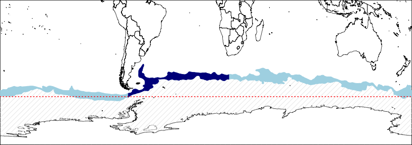
Map of various polygons computed here. In red, the 60°S parallel; in blue the Polar Frontal Zone (in dark blue, its Atlantic sector).