As it turned out, I realized the way I have been making maps in R since 10 years is more or less deprecated! Package sp was superseded by package sf, and indeed the coordinate system transformation works so much better and do not need as much weird hacking to work on complex projections. The code from last time thus become as follows:

library(sf)
system("gplates reconstruct -l /Applications/GPlates-1.5.0/SampleData/FeatureCollections/Coastlines/Shapefile/Seton_etal_ESR2012_Coastlines_2012.1_Polygon.shp \\
-r /Applications/GPlates-1.5.0/SampleData/FeatureCollections/Rotations/Seton_etal_ESR2012_2012.1.rot \\
-e shapefile -t 33.5 -o ~/Desktop/reconstructed")
coast <- read_sf("~/Desktop/reconstructed.shp") #This, already, is an improvement on the previous cumbersome readOGR

library(NSBcompanion)
nsb <- nsbConnect("guest","arm_aber_sexy")
exp113 <- dbGetQuery(nsb,"SELECT hole_id, paleo_latitude, paleo_longitude,rotation_source FROM neptune_paleogeography WHERE hole_id LIKE '113_%' AND reconstructed_age_ma=33.5;")
dbDisconnect(nsb)

dest_projection <- CRS("+proj=laea +lat_0=-90 +lon_0=0")
exp113pts <- st_multipoint(cbind(exp113$paleo_longitude, exp113$paleo_latitude),dim="XY") #Two-step approach, similar to what we had in "sp"
exp113sfc <- st_sfc(exp113pts,crs="+proj=longlat")
polar_113 <- st_transform(exp113sfc,dest_projection)
polar <- st_transform(coast,dest_projection)

limitANT <- st_sfc(st_linestring(cbind(-180:180,-45)),crs="+proj=longlat") #Way simpler here.
limitANT <- st_transform(limitANT,dest_projection)

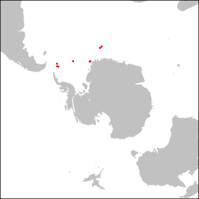
png("eocene2.png",h=400,w=400)
par(mar=c(0,0,0,0))
plot(limitANT,col="white")
plot(polar$geometry,col="grey80",border="grey80", add=TRUE)
plot(polar_113,col="red",pch=19,cex=0.5,add=TRUE)
box(lwd=3)
dev.off()

With the following result (identical to the one in the previous post obviously): Trying more complex, better projections is clearly seamless (though not trivial) but still have a few glitches that will need to taken care of:

dest_projection2 <- CRS("+proj=ortho +lat_0=-90 +lon_0=0") #Projection orthogonal, more natural
polar2_113 <- st_transform(exp113sfc,dest_projection2)
polar2 <- st_transform(coast,dest_projection2)

valids <- st_is_valid(polar2) # Some geometries fail with that projection unfortunately

png("eocene3.png",h=400,w=400)
par(mar=c(0,0,0,0))

#Draw a circle around earth
r <- 6400000 #earth radius
t <- seq(0,2*pi,by=0.01)
plot(r*cos(t),r*sin(t),col="black",lty=1,lwd=1.5,type="l")

plot(polar2[valids,]$geometry,col="grey80",border="grey80",add=TRUE)
plot(st_make_valid(polar2[!valids,]),col="grey80",border="grey80",add=T) #Yes, as simple as "make_valid" :)
plot(polar2_113,col="red",pch=19,cex=0.5,add=TRUE)

dev.off()

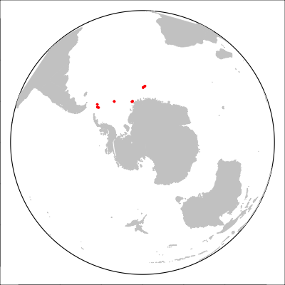
As one can see South America and Africa suffer from the projection: Hopefully I ll find a solution for that, at some point.