As promised in the first post of this series, I am going to show here how to use gplates to calculate the paleocoordinates of specific sites given a specific rotation model, using GPlates. To make it worth it, I'll use here the Matthews et al. 2016 rotation model as it is an update on the one we are using in the Neptune database. Also, and just for fun, we are going to compute the paleocoordinates of the two sites we drilled during Expedition 379 to the Amundsen Sea, an expedition I was part of. We only drilled until the latest Miocene but here I am going to compute the coordinates in the Turonian (as a tribute to the Klages et al. 2020 paper). The first step, as usual, is to get the sites current coordinates from Neptune (using my NSBcompanion package). I know that I mentioned in the previous post that rgdal/sp packages were obsolete and needed to be replaced with package sf, but I am not yet familiar enough with sf so here it is with rgdal/sp:

library(rgdal)
setwd("~/Desktop") #For code simplicity I am explicitely setting a working directory in which every file will be.
nsb <- NSBcompanion::nsbConnect("guest","arm_aber_sexy")
exp379 <- dbGetQuery(nsb,"SELECT hole_id, longitude, latitude FROM neptune_hole_summary WHERE leg=379 and hole='A';")
dbDisconnect(nsb)
exp379sp <- SpatialPointsDataFrame(exp379[,-1],data=exp379, proj4string=CRS("+proj=longlat"))
writeOGR(exp379sp,".","exp379",driver="ESRI Shapefile") #"." because we save it in the current folder

Then we'll download the data from the Matthews et al. 2016 paper from the EarthByte website (the makers of GPlates).

download.file("https://www.earthbyte.org/webdav/ftp/Data_Collections/Matthews_etal_2016_Global_Plate_Model_GPC.zip","Matthews_etal_2016.zip") #download
unzip("Matthews_etal_2016.zip") #unzip

Here we determine on which tectonic plates the sites we want to backtrack are:

system("gplates assign-plate-ids -p Matthews_etal_2016_Global_Plate_Model_GPC/Global_EarthByte_Mesozoic-Cenozoic_plate_boundaries_Matthews_etal.gpml\\
       -l exp379.shp -t 0 -s shapefile")
# -p is the plate boundary file that will be used to partition the sites
# -l is the feature we want to partition
# -t is the time at which the features are taken
# -s is the format we want to save the result as

# Just to check it worked, read in the file and check it has plate IDs
e3 <- readOGR(".","exp379")
e3$PLATEID1 #Should show 802 for both sites.
rm(e3)

Then we use the same method as previously to reconstruct the coastlines and the sites at the given time (here 90Ma):

system("gplates reconstruct -t 90 -l exp379.shp\\
       -r Matthews_etal_2016_Global_Plate_Model_GPC/Global_EB_250-0Ma_GK07_Matthews_etal.rot\\
       -o exp379_cretaceous -e shapefile")

system("gplates reconstruct -t 90 -l Matthews_etal_2016_Global_Plate_Model_GPC/StaticGeometries/Coastlines/Global_coastlines_2015_v1_low_res.shp \\
       -r Matthews_etal_2016_Global_Plate_Model_GPC/Global_EB_250-0Ma_GK07_Matthews_etal.rot\\
       -o coast_cretaceous -e shapefile")

And finally we plot them the exact same way as previously:

exp379cret <- readOGR(".","exp379_cretaceous")
coast <- readOGR(".","coast_cretaceous")

dest_projection <- CRS("+proj=laea +lat_0=-90 +lon_0=0")
polar <- spTransform(coast,dest_projection)
polar_379 <- spTransform(exp379cret,dest_projection)
polar_poly <- as(polar,"SpatialPolygons") #Here the coastlines are indeed lines, but we want them as polygons so that we can color-fill them.

limitANT <- Lines(list(Line(cbind(-180:180,-45))),ID="a")
limitANT <- SpatialLines(list(limitANT),proj4string=CRS("+proj=longlat"))
limitANT <- spTransform(limitANT,dest_projection)

png("turonian.png",h=400,w=400)
par(mar=c(0,0,0,0))
plot(limitANT,col="white")
plot(polar_poly,col="grey80",border="grey80",add=TRUE)
plot(polar_379,col="red",pch=19,add=TRUE,cex=0.5)
box(lwd=3)
dev.off()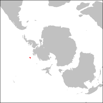

I know, it's a bit underwhelming since the Antarctic plate didn't move that much in the last 100Myr, but you get the gesture :)